STIP Retroactive Analysis – Yield Aggregators TVL
The below research report is also available in document format here .
TL;DR
In H2 2023, Arbitrum launched the Short-Term Incentive Program (STIP) by distributing millions of ARB tokens to various protocols to drive user engagement. This report focuses on how the STIP impacted TVL in the yield aggregator vertical, specifically examining the performance of Gamma, Jones DAO, Solv Protocol, Stella and Umami. By employing the Synthetic Control (SC) causal inference method to create a “synthetic” control group, we aimed to isolate the STIP’s effect from broader market trends. For each protocol the analysis focuses on the median TVL in the period from the first day of the STIP to two weeks after the STIP ended, in an effort to include at least two weeks of persistence in the analysis.
Yield aggregator protocols utilized their STIP allocations to incentivize depositors, leading to positive impacts on their TVL. Our analysis yielded varied results: Solv Protocol, Gamma, and Jones DAO experienced increases in their median TVL, directly attributed to the STIP, of $18.6M, $16.5M, and $12.6M, respectively, from the start of the STIP to two weeks after its conclusion. Stella and Umami also benefited, with $2.4M and $1M in additional TVL, respectively, linked to STIP incentives. During the STIP period and the two weeks following its conclusion, the added TVL per dollar spent on incentives was approximately $18 for Gamma, $5 for Jones DAO, $103 for Solv Protocol, $11 for Stella and $1 for Umami Finance. While the STIP positively impacted all protocols when considering the median TVL of the corresponding period, a different picture emerges when looking at growth from the program’s start to two weeks after its end. In this “before and after” comparison, the STIP slightly negatively impacted TVL growth for Solv Protocol (-8%) and had a minimal positive impact for Stella and Jones DAO (1%), even though Stella had a large TVL increase. In contrast, Umami experienced the most significant growth due to STIP, with a 120% increase (largely indirectly due to GMX’s grant), followed by Gamma with a 45% increase. It becomes clear that sustained growth, or “stickiness” is not correlated with each protocol’s success during the program. This is further underscored by comparing the growth with the TVL one month after the STIP, where all protocols experienced a much smaller increase. In every instance, the boost from incentives proved to be somewhat temporary, with only a small portion of the growth remaining a month after the STIP concluded.
The analysis indicates that direct incentives to LPs can yield substantial TVL growth and efficient use of funds. Flexibility in strategy also proved beneficial, as Umami Finance’s switch to direct ARB emissions significantly boosted their TVL. Stella’s balanced approach of splitting incentives between strategies and lending pools also led to a notable increase. Overall, the findings suggest that smaller protocols have more room for rapid growth when given substantial incentives, while larger protocols, like Solv Protocol, might benefit from a more proportional allocation to maximize efficiency. Protocols should reward users directly, uniformly over time, and transparently for providing liquidity while maintaining flexibility to adapt to feedback.
Our methodology and detailed results underscore the complexities of measuring such interventions in a volatile market, stressing the importance of comparative analysis to understand the true impact of incentive programs like STIP.

Context and Goals
In H2 2023, Arbitrum initiated a significant undertaking by distributing millions of ARB tokens to protocols as part of the Short-Term Incentive Program (STIP), aiming to spur user engagement. This program allocated varying amounts to diverse protocols across different verticals. Our objective is to gauge the efficacy of these recipient protocols in leveraging their STIP allocations to boost the usage of their products. The challenge lies in accurately gauging the impact of the STIP amidst a backdrop of various factors, including broader market conditions.
This report pertains to the yield aggregator vertical in particular. In this vertical, the STIP recipients were Gamma, Jones DAO, Solv Protocol, Stella and Umami. Stake DAO faced some KYC issues, which significantly delayed the start of the program. As a result, Stake DAO was only able to distribute incentives for three weeks concurrently with other protocols, and its distribution is still ongoing. The following table summarizes the amount of ARB tokens received and when they were used by each protocol.

For yield aggregators, TVL is a highly relevant metric. These protocols aim to facilitate “deploy and forget” strategies that minimize user interaction, making metrics like transactions or fees less pertinent. Throughout the report, the 7-day moving average (MA) TVL was used, so any mention of TVL should be understood as the 7-day MA TVL.
We used a Causal Inference method called Synthetic Control (SC) to analyze our data. This technique helps us understand the effects of a specific event by comparing our variable of interest to a “synthetic” control group. Here’s a short breakdown:
- Purpose: SC estimates the impact of a particular event or intervention using data over time.
- How It Works: It creates a fake control group by combining data from similar but unaffected groups. This synthetic group mirrors the affected group before the event.
- Why It Matters: By comparing the real outcomes with this synthetic control, we can see the isolated effect of the event.
In our analysis, we use data from other protocols to account for market trends. This way, we can better understand how protocols react to changes, like the implementation of the STIP, by comparing their performance against these market-influenced synthetic controls. The results pertain to the period from the start of each protocol’s use of the STIP until two weeks after the STIP had ended.
Results
Gamma
Gamma, a protocol specializing in active liquidity management and market-making strategies, offers non-custodial, automated, and active concentrated liquidity management services. Gamma is supported in fourteen different networks, including Arbitrum, where it launched November 1, 2022.
The STIP aimed to distribute ARB tokens to liquidity providers (LPs) who participated in qualified Gamma vaults. These vaults were built on the liquidity pools of six supported AMMs: Uniswap V3, Sushiswap V3, Ramses, Camelot, Zyberswap, and Pancakeswap. 100% of the incentives were allocated to LPs.
The primary objective of the program was to enhance liquidity on the Arbitrum network by deploying incentives on three native AMMs (Ramses, Camelot, and Zyberswap) and three non-native AMMs (Uniswap, Sushiswap, and Pancakeswap). Gamma engaged in discussions with partner AMMs to identify suitable pools to incentivize, focusing on under-capitalized pools based on their analysis of trading activity on the Arbitrum network.
Gamma’s methodology for selecting pairs considered various factors. It prioritized native pairs to Arbitrum, which typically required more liquidity and were under-capitalized. Critical infrastructure pairs, such as WETH, ARB, WBTC, and stablecoins, were also a focus, given their regular use by most users. Additionally, Gamma considered pairs that aligned with the strengths of the AMM they were on, while avoiding pairs already incentivized by other parties or overcapitalized ones. The incentive structure was designed to ensure that AMMs did not work against each other inefficiently. No matching funds for grant matching were available.

Gamma’s TVL grew from approximately $17.7M on November 15, 2023, when the STIP began, to around $43.4M at its peak in end January 2024. By the end of the STIP on March 20, 2024, the TVL was $38.0M. One week later, on March 27, the TVL was $35.3M, and two weeks after the STIP ended, on April 3, it dropped to $33.4M. By one month after the STIP concluded, on April 17, the TVL had decreased to $20.5M.
This represents a 114.2% increase in TVL from before the STIP to after it. Comparing the start of the STIP to the TVL one week after its end shows a 99.1% increase, while two weeks after the STIP ended, there was a 88.4% increase.
It’s worth noting that on January 4, 2024, Gamma temporarily halted deposits into their vaults due to an issue affecting four of the stable and LST vaults. Following OpenZeppelin’s investigation and their confirmation that Gamma’s mitigation was effective, deposits resumed on January 23rd.


The median impact of the STIP on Gamma’s TVL, from its start on November 15, 2023, to its end on March 20, 2024, was $16.2M. Including the TVL two weeks after the STIP concluded, the impact was $16.5M. Gamma received a total of 750k ARB, valued at approximately $900k (at $1.20 per ARB). This indicates that the STIP generated an average of $18.3 in TVL per dollar spent during its duration and the following two weeks. These results were gathered with 95% statistical significance.
Jones DAO
Jones DAO, a yield, strategy, and liquidity protocol, offers vaults that provide easy access to different strategies, aiming to enhance liquidity and capital efficiency for DeFi through yield-bearing tokens. In the STIP, Jones DAO requested 2 million ARB tokens to be allocated as follows: 82.5% for user incentives in current vaults and 17.5% for user incentives in future vaults.
A significant portion of these incentives was allocated to GLP-related products, while GMX focused on V2 growth in its program. Since future products were not released in time, all the incentives were ultimately distributed to existing products. Jones DAO’s execution strategy aimed to distribute 100% of the ARB allocation directly to Jones Vault users and the lending strategies built upon these vaults.
The distribution of ARB tokens was designed to align with the current yield distribution methods of Jones strategies. For instance, if a vault distributed yield weekly, ARB tokens would also be distributed weekly. Conversely, if yield distribution was constant, ARB tokens would be streamed continuously.
Jones DAO concluded that reducing the relative percentage of rewards per category and focusing more on integrations within the Arbitrum ecosystem, rather than solely on native farms, could enhance capital efficiency.

Jones DAO’s TVL grew from approximately $15.6M on November 28, 2023, when the STIP began, to around $30.7M at its peak in end January 2024. By the end of the STIP on March 29, 2024, the TVL was $25.2M. One week later, on April 5, the TVL was $18.2M, and two weeks after the STIP ended, on April 12, it dropped to $14.4M. By one month after the STIP concluded, on April 29, the TVL had decreased to $12.8M.
This represents a 61.8% increase in TVL from before the STIP to after it. Comparing the start of the STIP to the TVL one week after its end shows a 16.5% increase, while two weeks after the STIP ended, there was a 7.6% decrease.
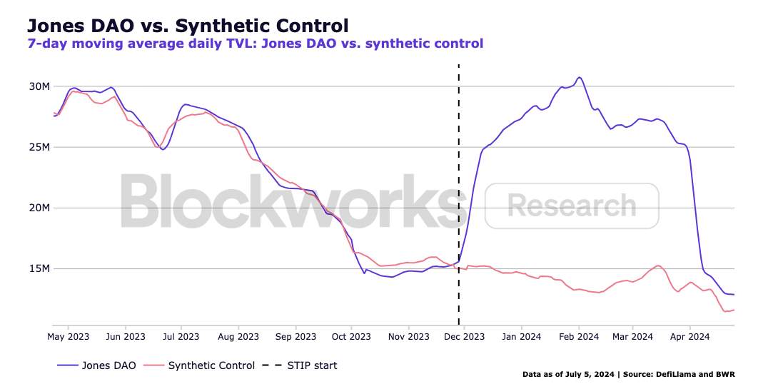
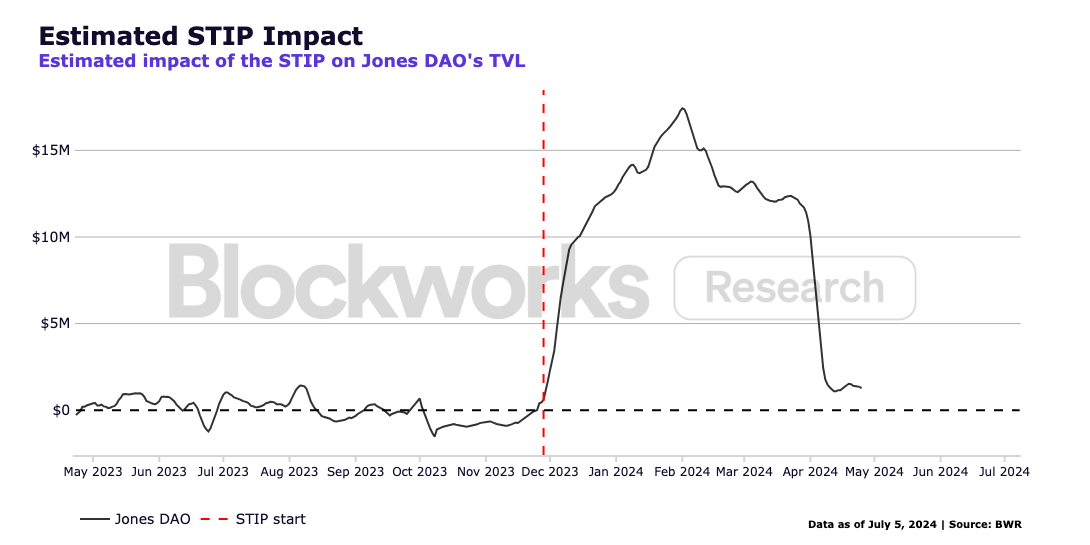
The median impact of the STIP on Jones DAO’s TVL, from its start on November 28, 2023, to its end on March 29, 2024, was $12.8M. Including the TVL two weeks after the STIP concluded, the impact was $12M. Jones DAO received a total of 2M ARB, valued at approximately $2.4M (at $1.20 per ARB). This indicates that the STIP generated an average of $5.25 in TVL per dollar spent during its duration and the following two weeks. These results were gathered with 95% statistical significance.
Solv Protocol
Solv Protocol has launched innovative products like Vesting Vouchers, Bond Vouchers, and Fund SFT for on-chain funds. Solv V3 offers a transparent platform where global institutions and retail investors can access a variety of trusted crypto investments. It also supports fund managers in raising capital and establishing on-chain credibility.
In the STIP, Solv Protocol planned to issue multiple DeFi market-making funds designed to provide users with consistent and appealing returns in a controlled environment with relatively low risk, exemplified by the open-end GMX fund with a $20,000,000 capacity. To enhance yield returns and bootstrap token governance, Solv incorporated a plan for token emissions, with the addition of ARB tokens aiming to attract high-value Arbitrum users.
100% of the allocated ARB (150,000 ARB) was designated as extra incentives for fund products on Solv Arbitrum, split equally between Offchain/RWA funds and Onchain Delta Neutral Strategy funds. The ARB incentives were proportionally allocated among users based on their cumulative daily holdings across vaults on Arbitrum. These incentives were airdropped directly to Solv vault investors after the completion of each of the three distribution epochs.
Additionally, Solv Protocol confirmed its commitment to grant matching with future token issuance.

Solv Protocol’s TVL grew from approximately $71.3M on January 1, 2024, when the STIP began, to around $122.6M at its peak in March 2024. By the end of the STIP on March 29, 2024, the TVL was $106.1M. One week later, on April 5, the TVL was $105.2M, and two weeks after the STIP ended, on April 12, $105.9M. By one month after the STIP concluded, on April 26, the TVL had decreased to $89.7M.
This represents a 48.8% increase in TVL from before the STIP to after it. Comparing the start of the STIP to the TVL one week after its end shows a 47.5% increase, while two weeks after the STIP ended, the increase remained steady around 48.5%.


The median impact of the STIP on Solv Protocol’s TVL, from its start on January 1, 2024, to its end on March 29, 2024, was $25.1M. Including the TVL two weeks after the STIP concluded, the impact was $18.6M. Solv Protocol received a total of 150k ARB, valued at approximately $180k (at $1.20 per ARB). This indicates that the STIP generated an average of $103.5 in TVL per dollar spent during its duration and the following two weeks. These results were gathered with 90% statistical significance.
Stella
Stella, a leveraged yield farming protocol on Arbitrum, offers 0% cost to borrow and enables leveraged strategies on yield sources like Uniswap DEXs, TraderJoe liquidity book, and the Pendle PT pools.
The protocol is divided into two parts: Stella Strategies (leveraged strategies) and Stella Lend (lending pools). A total of 186,000 ARB tokens were allocated as incentives, distributed between these two parts as follows:
- Approximately 66,000 ARB tokens were designated for Stella Strategies, providing an additional 20% yield for profitable leveraged positions. This incentive was exclusive to profitable positions to prevent sybil attacks and encourage good behavior.
- Around 120,000 ARB tokens were allocated to Stella Lending pools. The exact incentive amount for each pool was determined dynamically based on what seemed appropriate.
Stella aimed to stimulate both the strategy and lending sides, initiating a positive feedback loop for growth.
According to Stella, this experience highlighted the need to adjust protocol mechanics to make lending more attractive, as the borrow capacity was consistently maxed out while lending liquidity lagged. To address this, Stella implemented an “airdrop points sharing” system where lenders earned 50% of points from EigenLayer and LRT, enhancing the appeal of lending.
The ARB incentives were distributed innovatively. For Stella Strategies, the incentives were auto-deposited into the ARB lending pool on Stella with a linear vesting period of 30 days, preventing immediate dumping and allowing leverage users to earn additional lending yields over this period. This approach also helped bootstrap liquidity in the ARB lending pool, benefiting both the lending and leveraged farming sides.

Stella’s TVL grew from approximately $2.3M on November 3, 2023, when the STIP began, to around $9.3M at its peak in March 2024. By the end of the STIP on March 29, 2024, the TVL was $7.2M. One week later, on April 5, the TVL was $6.0M, and two weeks after the STIP ended, on April 12, it dropped to $5.1M. By one month after the STIP concluded, on April 29, the TVL had decreased to $3.8M.
This represents a 211.3% increase in TVL from before the STIP to after it. Comparing the start of the STIP to the TVL one week after its end shows a 158.9% increase, while two weeks after the STIP ended, the increase was 120.5%.


The median impact of the STIP on Stella’s TVL, from its start on November 3, 2023, to its end on March 29, 2024, was $2.5M. Including the TVL two weeks after the STIP concluded, the impact was $2.4M. Stella received a total of 186k ARB, valued at approximately $223k (at $1.20 per ARB). This indicates that the STIP generated an average of $10.8 in TVL per dollar spent during its duration and the following two weeks. These results were gathered with 95% statistical significance.
Umami Finance
Umami Finance implemented an oARB emissions tool, inspired by Dolomite’s system, to distribute their STIP allocation. This tool allowed users to stake their Umami vault receipt tokens for oARB emissions, which were continuously emitted and could be vested on a first-come, first-served basis. The emitted oARB could be staked for a duration of up to four months, in weekly increments, paired with an equal amount of ARB. After the vesting period, users could obtain the underlying ARB at a discounted price, with the discount increasing by 2.5% per additional week staked, subject to change based on feedback. However, if the ARB rewards pool was depleted, all remaining oARB tokens would expire worthless. The staked ARB paired with oARB was deposited back into Umami to improve capital efficiency for farmers.
The implementation of oARB emissions faced challenges, particularly with the availability of ARB from vesting contracts. While early depositors initially enjoyed high returns, issues arose towards the end of the period as more users opted for the non-ETH investment 40-week option, necessitating a tapering of emissions. Looking ahead, Umami Finance decided to adopt a direct incentive approach with dynamic incentives, instead of the oARB incentive mechanism.
Umami Finance also used GMX’s grant of 100,000 ARB, and so was able to delay ARB yield from the STIP and utilize direct ARB emissions with the GMX grant for 45 days. 702,775 ARB was distributed through the scaling GLP vaults with the oARB emissions program, which concluded on January 26th. After this, the remaining 47,225 tokens from the STIP together with GMX’s 100k ARB were allocated to GM Vault direct emissions.

Umami’s TVL grew from approximately $3.3M on November 13, 2023, when the STIP began, to around $11.2M at its peak in February 2024. By the end of the STIP on March 29, 2024, the TVL was $10.5M. One week later, on April 5, the TVL was $11.1M, and two weeks after the STIP ended, on April 12, it dropped to $10.6M. By one month after the STIP concluded, on April 29, the TVL was at $10.7M.
This represents a 220.8% increase in TVL from before the STIP to after it. Comparing the start of the STIP to the TVL one week after its end shows a 238.6% increase, while two weeks after the STIP ended, the increase was 223.7%.


The median impact of the STIP on Umami’s TVL, from its start on November 13, 2023, to its end on March 29, 2024, was $726.7k. Including the TVL two weeks after the STIP concluded, the impact was $1.2M. Umami Finance received a total of 750k ARB, valued at approximately $900k (at $1.20 per ARB). This indicates that the STIP generated an average of $1.2 in TVL per dollar spent during its duration and the following two weeks. These results were gathered with 95% statistical significance.
Main Takeaways
Our analysis produced interesting results for the impact of the STIP on Gamma, Jones DAO, Solv Protocol, Stella and Umami. The table below summarizes these results. A further explanation of how this and all results were derived can be found in the Methodology section.
A summary of the key differentiators in incentive allocation is shown in the table below.

All yield aggregator protocols used the STIP allocation to provide direct incentives to their depositors, resulting in a positive impact on their TVL. Notably, these protocols vary significantly in the products they offer and their operational methods. While diversity exists in other DeFi verticals as well, it is particularly pronounced among yield aggregators. For instance, although classified as yield aggregators within the context of STIP and the Arbitrum DAO, entities like DefiLlama categorize them differently, including them in various verticals such as yield protocols, liquidity managers, RWA, and leveraged farming.
Smaller protocols like Stella (starting at $2.3M) and Umami ($3.3M) saw the largest TVL increases from the start of the STIP to their respective peak TVLs. However, Umami maintained its TVL increase in a much steadier fashion even two weeks after the STIP. While the STIP generated a 120% TVL growth for Umami, Stella only saw a 1% increase in this period. Despite this, with Umami’s grant size being four times that of Stella, the efficiency of the STIP in terms of median TVL added per dollar was much higher for Stella, at $10.83 compared to Umami’s $1.20. This median TVL considers the entire duration of the STIP plus two weeks post-STIP.
Gamma’s TVL growth from start to peak was the third largest, further supporting the idea that smaller protocols benefit proportionally more from the program. Nearly all of Gamma’s growth, 116%, can be attributed to the STIP, compared to its total growth of 145%. Even considering the growth from start to two weeks after the STIP’s end, the 45% increase attributed to the STIP is significant. Gamma’s median added TVL attributed to the STIP was $18.33 per dollar spent, higher than both Stella and Umami due to its efficient allocation.
Jones DAO started with a TVL similar to Gamma but experienced less growth from start to peak, with a 55% increase attributed to the STIP during this period. Notably, there was a decrease in TVL when comparing two weeks post-STIP to the pre-STIP period. However, the STIP still had a positive impact, albeit small, of 1%. The median TVL added by the STIP was $12.6M, resulting in $5.25 TVL per dollar, which is on the lower end for this group. The team concluded that focusing more on integrations within the Arbitrum ecosystem, rather than solely on native farms, could enhance capital efficiency.
Solv Protocol began the STIP with nearly five times the TVL of Jones DAO or Gamma, yet still saw a comparable increase of 48.6% during the STIP period and two weeks after. Although the absolute median TVL added was the largest, it wasn’t substantially higher than Gamma or Jones DAO when considering the higher starting point. Our analysis reveals an 8% TVL decrease attributed to the STIP in the period after two weeks and only a 2% increase at its peak TVL. This suggests that while the STIP initially boosted growth, it stagnated towards the end. This stagnation might be due to the uneven distribution method over three epochs, with the first batch of incentives released only on March 5, 2024, after three months of user participation. The two remaining batches were all distributed within March. Despite this, Solv Protocol achieved a median of $103.47 added TVL per dollar spent. Notably, Solv’s allocation was the smallest at 150k ARB, similar to Stella’s 186K ARB and much smaller than Jones DAO’s 2M ARB. A more proportional allocation might have enabled the protocol to perform better.
Direct incentives to LPs seem effective: Gamma, which allocated 100% of incentives directly to LPs, saw a significant TVL impact and a good TVL per dollar spent ratio. Diversified incentive allocation can also be beneficial: Stella, which split incentives between strategies and lending pools, achieved the highest TVL increase and a high STIP impact. This indicates that a balanced approach targeting different aspects of the protocol can yield positive results.
Flexibility and adaptability are crucial: Umami Finance’s experience demonstrates that adjusting strategies—such as switching from oARB emissions to direct ARB emissions—can lead to significantly better results. They saw the highest impact on their TVL after this change, indicating that direct emissions are much better received than strategies involving lock and vesting, like oARB. The substantial increase in TVL attributed to the STIP two weeks after its end, which includes the GMX grant, highlights this point. However, because Umami’s initial allocation was quite large, especially compared to similarly sized protocols like Stella, the efficiency measured by added TVL per dollar was relatively low.
The analysis suggests that smaller protocols might have more room for rapid growth when given significant incentives. However, while smaller protocols showed higher percentage overall growth, larger protocols often saw more significant absolute increases in TVL per dollar spent. This is an important distinction when evaluating the impact of incentives. A more proportional allocation of incentives might have enhanced the efficiency of distribution, as evidenced by Solv Protocol’s high added TVL per dollar compared to Umami’s lower efficiency.
Overall, the most successful approaches appear to be those that directly, uniformly over time and transparently reward users for providing liquidity, while maintaining the flexibility to adapt to changing market conditions or user behaviors. Protocols that can balance simplicity with strategic allocation across their ecosystem seem to achieve the best results in terms of TVL growth and efficient use of incentives.
It’s also interesting to note that most protocols’ TVL, normalized by ARB allocation, converges to values between $5 and $18 per ARB spent. Solv Protocol is an outlier due to its disproportionate allocation relative to its size. This indicates that, while the liquidity benefit of one ARB spent varies significantly throughout the program, the long-term benefit remains fairly consistent across most yield aggregators.

Methodology
TLDR: We employed an analytical approach known as the Synthetic Control (SC) method. The SC method is a statistical technique utilized to estimate causal effects resulting from binary treatments within observational panel (longitudinal) data. Regarded as a groundbreaking innovation in policy evaluation, this method has garnered significant attention in multiple fields. At its core, the SC method creates an artificial control group by aggregating untreated units in a manner that replicates the characteristics of the treated units before the intervention (treatment). This synthetic control serves as the counterfactual for a treatment unit, with the treatment effect estimate being the disparity between the observed outcome in the post-treatment period and that of the synthetic control. In the context of our analysis, this model incorporates market dynamics by leveraging data from other protocols (untreated units). Thus, changes in market conditions are expected to manifest in the metrics of other protocols, thereby inherently accounting for these external trends and allowing us to explore whether the reactions of the protocols in the analysis differ post-STIP implementation.
To achieve the described goals, we turned to causal inference. Knowing that “association is not causation”, the study of causal inference lies in techniques that try to figure out how to make association be causation. The classic notation of causality analysis revolves around a certain treatment ![]() , which doesn’t need to be related to the medical field, but rather is a generalized term used to denote an intervention for which we want to study the effect. We typically consider
, which doesn’t need to be related to the medical field, but rather is a generalized term used to denote an intervention for which we want to study the effect. We typically consider ![]() the treatment intake for unit i, which is 1 if unit i received the treatment and 0 otherwise. Typically there is an
the treatment intake for unit i, which is 1 if unit i received the treatment and 0 otherwise. Typically there is an ![]() , the observed outcome variable for unit i. This is our variable of interest, i.e., we want to understand what the influence of the treatment on this outcome was. The fundamental problem of causal inference is that one can never observe the same unit with and without treatment, so we express this in terms of potential outcomes. We are interested in what would have happened in the case some treatment was taken. It is common to call the potential outcome that happened the factual, and the one that didn’t happen, the counterfactual. We will use the following notation:
, the observed outcome variable for unit i. This is our variable of interest, i.e., we want to understand what the influence of the treatment on this outcome was. The fundamental problem of causal inference is that one can never observe the same unit with and without treatment, so we express this in terms of potential outcomes. We are interested in what would have happened in the case some treatment was taken. It is common to call the potential outcome that happened the factual, and the one that didn’t happen, the counterfactual. We will use the following notation:
![]() - the potential outcome for unit i without treatment
- the potential outcome for unit i without treatment
![]() - the potential outcome for the same unit i with the treatment.
- the potential outcome for the same unit i with the treatment.
With these potential outcomes, we define the individual treatment effect to be ![]() . Because of the fundamental problem of causal inference, we will actually never know the individual treatment effect because only one of the potential outcomes is observed.
. Because of the fundamental problem of causal inference, we will actually never know the individual treatment effect because only one of the potential outcomes is observed.
One technique used to tackle this is Difference-in-Difference (or diff-in-diff). It is commonly used to analyze the effect of macro interventions such as the effect of immigration on unemployment, the effect of law changes in crime rates, but also the impact of marketing campaigns on user engagement. There is always a period before and after the intervention and the goal is to extract the impact of the intervention from a general trend. Let ![]() be the potential outcome for treatment D on period T (0 for pre-intervention and 1 for post-intervention). Ideally, we would have the ability to observe the counterfactual and estimate the effect of an intervention as:
be the potential outcome for treatment D on period T (0 for pre-intervention and 1 for post-intervention). Ideally, we would have the ability to observe the counterfactual and estimate the effect of an intervention as: ![]() #0), the causal effect being the outcome in the period post-intervention in the case of a treatment minus the outcome in the same period in the case of no treatment. Naturally,
#0), the causal effect being the outcome in the period post-intervention in the case of a treatment minus the outcome in the same period in the case of no treatment. Naturally, ![]() is counterfactual so it can’t be measured. If we take a before and after comparison,
is counterfactual so it can’t be measured. If we take a before and after comparison, ![]() -E%5BY(0)%7CD%3D1)#0) we can’t really say anything about the effect of the intervention because there could be other external trends affecting that outcome.
-E%5BY(0)%7CD%3D1)#0) we can’t really say anything about the effect of the intervention because there could be other external trends affecting that outcome.
The idea of diff-in-diff is to compare the treated group with an untreated group that didn’t get the intervention by replacing the missing counterfactual as such: ![]() . We take the treated unit before the intervention and add a trend component to it, which is estimated using the control
. We take the treated unit before the intervention and add a trend component to it, which is estimated using the control ![]() . We are basically saying that the treated unit after the intervention, had it not been treated, would look like the treated unit before the treatment plus a growth factor that is the same as the growth of the control.
. We are basically saying that the treated unit after the intervention, had it not been treated, would look like the treated unit before the treatment plus a growth factor that is the same as the growth of the control.
An important thing to note here is that this method assumes that the trends in the treatment and control are the same. If the growth trend from the treated unit is different from the trend of the control unit, diff-in-diff will be biased. So, instead of trying to find a single untreated unit that is very similar to the treated, we can forge our own as a combination of multiple untreated units, creating a synthetic control.
That is the intuitive idea behind using synthetic control for causal inference. Assuming we have ![]() units and unit 1 is affected by an intervention. Units
units and unit 1 is affected by an intervention. Units ![]() are a collection of untreated units, that we will refer to as the “donor pool”. Our data spans T time periods, with
are a collection of untreated units, that we will refer to as the “donor pool”. Our data spans T time periods, with ![]() periods before the intervention. For each unit j and each time t, we observe the outcome
periods before the intervention. For each unit j and each time t, we observe the outcome ![]() . We define
. We define ![]() as the potential outcome without intervention and
as the potential outcome without intervention and ![]() the potential outcome with intervention. Then, the effect for the treated unit
the potential outcome with intervention. Then, the effect for the treated unit ![]() at time t, for
at time t, for ![]() is defined as
is defined as ![]() . Here
. Here ![]() is factual but
is factual but ![]() is not. The challenge lies in estimating
is not. The challenge lies in estimating ![]() .
.

Source: 15 - Synthetic Control — Causal Inference for the Brave and True
Since the treatment effect is defined for each period, it doesn’t need to be instantaneous, it can accumulate or dissipate. The problem of estimating the treatment effect boils down to the problem of estimating what would have happened to the outcome of the treated unit, had it not been treated.
The most straightforward approach is to consider that a combination of units in the donor pool may approximate the characteristics of the treated unit better than any untreated unit alone. So we define the synthetic control as a weighted average of the units in the control pool. Given the weights ![]() the synthetic control estimate of
the synthetic control estimate of ![]() is
is ![]() .
.
We can estimate the optimal weights with OLS like in any typical linear regression. We can minimize the square distance between the weighted average of the units in the donor pool and the treated unit for the pre-intervention period. Hence, creating a “fake” unit that resembles the treated unit before the intervention, so we can see how it would behave in the post-intervention period.
In the context of our analysis, this means that we can include all other yield aggregator protocols that did not receive the STIP in our donor pool and estimate a “fake”, synthetic, control yield aggregator protocol that follows the trend of any particular one we want to study in the period before receiving the STIP. As mentioned before, the metric of interest chosen for this analysis was TVL and, in particular, we calculated the 7-day moving average to smooth the data. Then we can compare the behavior of our synthetic control with the factual and estimate the impact of the STIP by taking the difference. We are essentially comparing what would have happened, had the protocol not received the STIP with what actually happened.
However, sometimes regression leads to extrapolation, i.e., values that are outside of the range of our initial data and can possibly not make sense in our context. This happened when estimating our synthetic control, so we constrained the model to do only interpolation. This means we restrict the weights to be positive and sum up to one so that the synthetic control is a convex combination of the units in the donor pool. Hence, the treated unit is projected in the convex hull defined by the untreated unit. This means that there probably won’t be a perfect match of the treated unit in the pre-intervention period and that it can be sparse, as the wall of the convex hull will sometimes be defined only by a few units. This works well because we don’t want to overfit the data. It is understood that we will never be able to know with certainty what would have happened without the intervention, just that under the assumptions we can make statistical conclusions.
Formalizing interpolation, the synthetic control is still defined in the same way by ![]() . But now we use the weights
. But now we use the weights ![]() that minimize the square distance between the weighted average of the units in the donor pool and the treated unit for the pre-intervention period
that minimize the square distance between the weighted average of the units in the donor pool and the treated unit for the pre-intervention period ![]() , subject to the restriction that
, subject to the restriction that ![]() are positive and sum to one.
are positive and sum to one.
We get the optimal weights using quadratic programming optimization with the described constraints on the pre-STIP period and then use these weights to calculate the synthetic control for the total duration of time we are interested in. We initialized the optimization for each analysis with different starting weight vectors to avoid introducing bias in the model and getting stuck in local minima. We selected the one that minimized the square difference in the pre-intervention period.
As an example, below is the resulting chart for Gamma, showing the factual TVL observed in Gamma and the synthetic control.
With the synthetic control, we can then estimate the effect of the STIP as the gap between the factual protocol TVL and the synthetic control, ![]() .
.
To understand whether the result is statistically significant and not just a possible result we got due to randomness, we use the idea of Fisher’s Exact Test. We permute the treated and control units exhaustively by, for each unit, pretending it is the treated one while the others are the control. We create one synthetic control and effect estimates for each protocol, pretending that the STIP was given to another protocol to calculate the estimated impact for this treatment that didn’t happen. If the impact in the protocol of interest is sufficiently larger when compared to the other fake treatments (“placebos”), we can say our result is statistically significant and there is indeed an observable impact of the STIP on the protocol’s TVL. The idea is that if there was no STIP in the other protocols and we used the same model to pretend that there was, we wouldn’t see any impact.
References
“Hernán MA, Robins JM (2020). Causal Inference: What If. Boca Raton: Chapman & Hall/CRC.”
Aayush Agrawal - Causal inference with Synthetic Control using Python and SparseSC
01 - Introduction To Causality — Causal Inference for the Brave and True